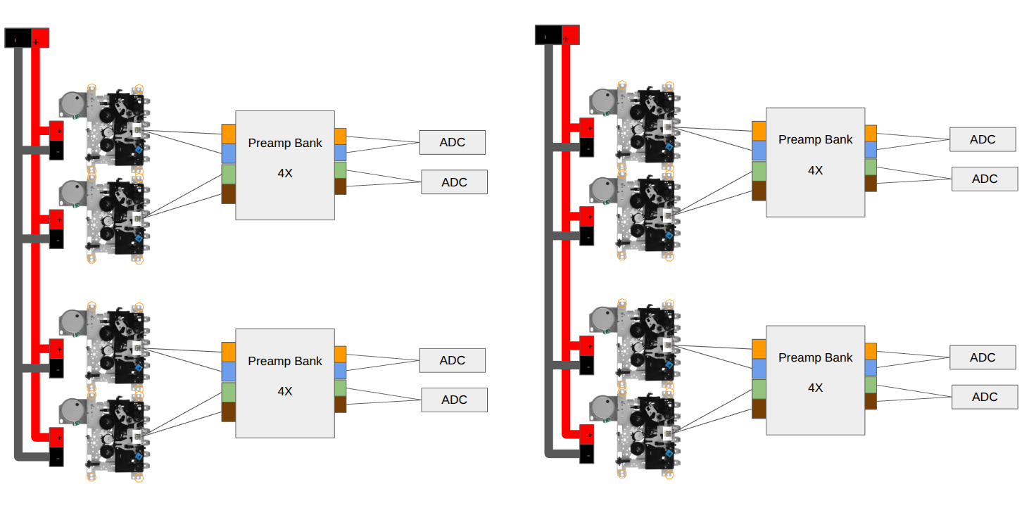
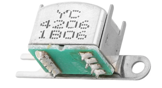
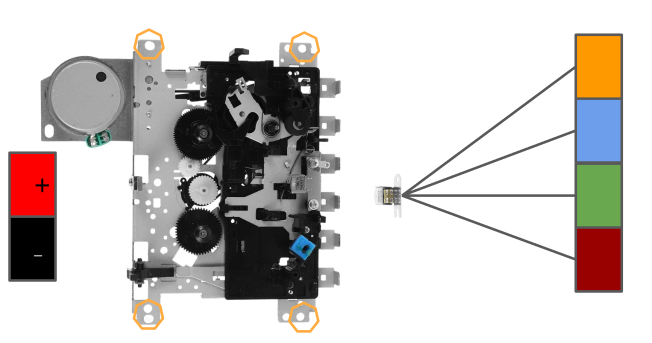
Requires Tape Flip
Requres Polarity Inversion:
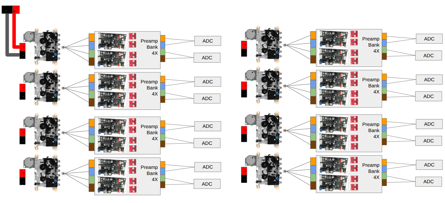
Singe Tape – TA7668 magnetic head Preamp with Dolby Class C and Dolby Class B
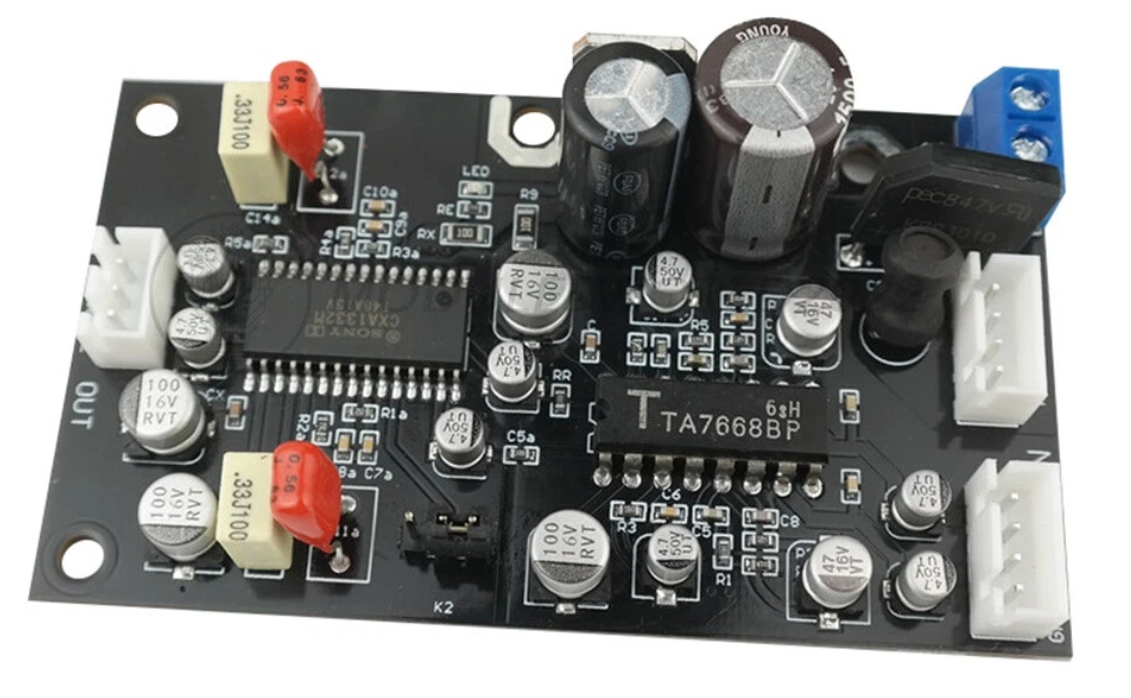

Requires Tape Flip
Requres Polarity Inversion:
Singe Tape – TA7668 magnetic head Preamp with Dolby Class C and Dolby Class B
There is a quiet, vanishing geometry to the way things used to be built. Spend a few days in a workshop with Richard Hess, listening to him talk through the microscopic behaviors of a tape path, and you realize that a tape machine isn’t just an electronic box that happens to have moving parts—it is an intricate mechanical instrument where physics and signal path are entirely inseparable.
For decades, the world has been sliding away from this reality. We live in an era of surface-mount components, sealed modules, and software emulations where physical touch has been engineered out of daily life. But in the trenches of analog audio, and particularly in the specialized world of tape preservation and high-end mastering, the physical world still demands absolute obedience.

Lately, I’ve found myself standing at a wonderful intersection. By combining a lifelong obsession with audio, a deep love for mechanical machining, and a practical foundation in electronics design, I’ve found a path forward that feels almost anachronistic, yet desperately needed. I am stepping into the world of custom headblock mechanics—machining bespoke mounts, zero-backlash adjustment platforms, and engineering the precise spatial relationships required to make tape heads sing.
Richard’s mentorship underscored a fundamental truth: you can have the finest electronics in the world, but if your azimuth is off by a fraction of a micron, or if your headblock flexes under the tension of a 10.5-inch reel, your high frequencies vanish into phase cancellation. The art is entirely mechanical. It is about cutting custom clearance holes in vintage castings, designing kinematic adjustment linkages that don’t bind, and selecting materials that refuse to thermal-drift when a studio heats up. It is about hand-lapping, micro-adjusting, and treating a piece of aluminum like a Swiss watch movement.
There is a massive opportunity hidden in this niche. Studios and archivists are guarding aging Studers, Ampexes, and MCI transports like holy relics. They don’t just need service; they need custom mechanical evolution—tailored modifications, specialized head configurations, and modern engineering applied to vintage iron.
By marrying the tactile grit of machining with the exact science of audio and electronics, I get to build things that matter. It’s a craft where the chips flying off the mill directly translate to the air moving out of a studio monitor, bridging the physical and the sonic in a way very few people still know how to do.
Bringing Hardware Sampler Soul to the Web Browser
The Web Sampler & Sequencer is a fully-featured, open-source drum machine designed to run entirely within a modern web browser. By bridging the tactile workflow of classic beat-making hardware with the accessibility of modern web APIs, it offers a robust music production experience directly from a web browser.
Here is a breakdown of what makes this project technically unique and how it faithfully honors its hardware roots.
The application stands out due to its radical approach to software architecture and browser integration, prioritizing transparency and local execution over cloud dependencies.
Zero-Dependency Architecture: The app requires no backend server, no Node.js environment, and no build tools like Webpack.
Direct Local File Access: It utilizes the File System Access API on Chromium-based browsers to let users browse and load samples directly from a local computer folder.
Absolute Privacy: Because it runs entirely client-side, the app never uploads a user’s audio files or patterns to a remote server.
Custom Legacy Audio Decoding: Alongside standard native Web Audio API formats (WAV, MP3, OGG, FLAC), it features a custom pure-JavaScript decoder for AIFF/AIFC files, which are common in vintage sample libraries.
Offline Independence: A built-in service worker caches the application shell and libraries, allowing the sampler to function completely offline after the initial load.
Transparent Codebase: The source code adheres to a strict philosophy where no individual file exceeds 200 lines.
No Compilation Needed: The app runs React natively in the browser via standalone Babel, meaning anyone can “View Source,” edit the code in a text editor, and refresh the page to see changes immediately.
Despite running in a web browser, the application meticulously recreates the physical feel and workflow limitations that made classic hardware samplers so intuitive.
 Classic MPC Layout: The interface is built around a traditional 4×4 grid of 16 drum pads.
 Mouse-Based Velocity: It simulates physical velocity sensitivity by calculating how close the user clicks to the exact center of a pad.
 Plug-and-Play MIDI: The Web MIDI API allows users to plug in class-compliant USB controllers (like an Akai MPD) to finger-drum immediately with real velocity capture.
 Tone Mode: By holding
 CTRL and clicking a pad, users can map a single sample chromatically across all 16 pads to sequence melodies and basslines.
 Advanced Step Sequencing: The sequencer mimics classic hardware parameters, offering granular, per-step control over velocity, panning, pitch, and swing (shuffle).


 Analog-Modeled Synthesis: When no sample is loaded on a pad, the app falls back on custom synthesis engines designed to strip acoustic percussion down to its physics—such as modeling the thump of a kick drum or the high-pass filtered noise of a snare wire.
| Hardware Concept | Web Sampler Implementation |
| Internal Memory |
Saves kits, favored samples, and patterns locally using browser |
| Sample Browsing |
Recursively scans local directories to build a searchable, visual waveform grid. |
| Pattern Chaining |
Provides 4, 8, 16, 32, and 64-step pattern options that can be managed in a dedicated Song tab. |
| Mixer Console |
Features a dedicated mixer view with per-track volume, panning, and a shared reverb bus.
|

At its core, scanalyzer is a smart, automated librarian for your audio files. If you have a massive, unorganized folder full of thousands of random audio samples,
finding the exact sound you need can be a nightmare. This software “listens” to every single file, figures out what it actually sounds like, and visually organizes
your entire collection so you can browse it instantly.
Instead of relying on whatever messy name the file was given (like BD_01_final_v2.wav ), the tool relies on acoustic science. When you point it at a folder, it does
the following:
1. Listens & Measures: It quickly scans through your audio files and measures things like how loud it is, how long it rings out, whether it’s a pitched note (like a
piano) or a burst of noise (like a cymbal), and how distorted it is.
2. Classifies & Groups: Based on those measurements, it categorizes the sound. It can tell the difference between a thumping bass, a short drum hit, a lingering
background texture, or a vocal line. It organizes them into a top-level hierarchy (like Percussive, Tonal, or Complex).
3. Builds a Map: It groups sounds that share similar characteristics together—regardless of what they are named.
• The 3D Sound Cloud: It takes all your sounds and plots them as points in a 3D interactive “cloud.” You can literally see your entire sample library at a glance. If
you click an area where the “kick drums” are grouped, you can visually explore and play similar sounds right next to each other.
• Intelligent Renaming & Reorganizing: Once the software knows what everything is, it features a tool that allows you to easily rename your files and sort them into
neat, structured folders based on their true acoustic traits.
• 100% Private (No Cloud Needed): Even though there is a web browser version of this app, none of your audio files ever leave your computer. All the heavy lifting is
done right on your machine, so your private library stays private.
• Never Scans the Same Thing Twice: Once a file is scanned, it creates a tiny digital “nametag” (a .PEAK file) next to it. If you run the scan again in the future,
it reads the nametag instead of re-listening to the whole sound, saving you a ton of time.
You can use the tool in two ways—they both do the exact same thing:
• As a Desktop App: A standalone application window running on your computer.
• As a Web Page: A sleek web interface that runs right in your browser (but again, totally offline and client-side).
It turns a chaotic, messy folder of audio files into a clean, searchable, visually explorable library using the actual sound of the files, not just their
filenames.


A browser-based broadcast signal routing visualizer, dressed in full LCARS regalia.
It maps the living signal flow of a multi-floor production facility — every stage box,
every camera, every audio channel — onto destinations like control rooms, edit suites,encoders, and floor rooms. You drag a source onto a destination’s input, and the patchcomes alive as a twisting strand of DNA.
The “twist” is the metaphor and the mechanic: each routing point is a twist, and thesignals you braid into it are rendered as an animated double helix — two strands (cyan and magenta) spiraling around each other, the way two feeds wind together into one production.
Route a healthy source and the helix flows clean; route a faulted one and the strand corrupts, flickering red.

Sources (left ingress panel) — draggable signal nodes, discovered dynamically from theSources/ tree:

Destinations (footer tabs) — consumers of signal, discovered from the Destinations/
tree. Each category (Control Rooms, Edit Suites, Encoders, Floors…) becomes a tab group;
each room is a tab full of twists:

Patching — drag a source onto a twist. The twist’s helix grows to show what’s braided
in; click the LCARS lip or the left bar to fold/unfold the strand. Open a twist to get a
matrix modal where you drag rows to reorder priority and switcher-input assignments.
Fault propagation — any source whose status isn’t OK (e.g. LOST CLOCK) pulses red.
Route it anywhere and the destination inherits the alarm: the room’s LCARS L-bar pulses red
and the twist’s DNA strand corrupts. Faults are visible end-to-end, the way they should be
in a real plant.
Zero-backend discovery — the whole source/destination tree is just folders of JSON.
Drop in a new stage box or a new control room and it appears in the UI; no code change.
Discovery prefers an index.json manifest in each folder (so it works on any static
host), and falls back to parsing autoindex HTML when none is present.
Data model
Everything is plain JSON under two roots:
Sources/        # draggable signals
  Audio/<Floor>/<box>.json
  Video/<Floor>/<box>.json
  Productions/<program>.json
Destinations/   # twists that consume signal
  Control Rooms/<tier>/<room>.json
  Edit Suites/<suite>.json
  Encoders/<encoder>.json
  Floors/<floor>/<room>.json
A source declares its channels, a colour class, a floor, and a status:
{ "id": "stagebox-101", "name": "STAGEBOX 101", "prefix": "S101-", "count": 12,
  "extraClass": "audio-studio", "floor": "1st Floor", "items": ["CH 1", "…"],
  "status": "LOST CLOCK" }
A destination declares its twists, each with what it accepts (video / audio /both), its switcher inputs, and limits like maxVideo / maxAudio:
{ "id": "prod3", "name": "PROD 3", "color": "#646DCC",
  "twists": [ { "name": "Video Mixer", "accepts": "video", "inputs": ["SW IN 1", "…"] } ] }
Local, no dependencies (uses Python’s stdlib server, which provides the autoindex fallback):
python3 start.py # serves the UI and opens your browser on a free port
Deploy to a static host over FTPS:
python3 uploadftp.py # regenerates every index.json manifest, then uploads only the git diff
uploadftp.py is the smart deployer: it walks Sources/ and Destinations/ writing freshindex.json manifests, then uses git status to upload only what changed (handling
renames and deletions), falling back to a full upload when there’s no diff. FTP credentials
come from a local .env (FTP_HOST, FTP_USER, FTP_PASS). (deploy.py is the older,
simpler full-tree uploader.)
The app is plain HTML/CSS/JS — no framework, no build step:
index.htm            # shell + all the LCARS styling
js/globals.js        # discovery (listDirectory/fetchJSON), folding, tabs
js/poolVideo.js      # render video source pools
js/poolAudio.js      # render audio source pools
js/visuals.js        # the DNA-helix SVG rendering
js/matrix.js         # twists, routing, the matrix modal, fault logic
js/dragDrop.js       # drag-and-drop patching
js/productions.js    # productions-as-sources
js/topbar.js         # destination tabs / groups
js/app.js            # boot: build the tree, wire everything up
This project is a love letter to LCARS — the Library Computer Access/Retrieval System — the operating-system aesthetic of the 24th century. None of this look would exist without the artists who invented it:
The colours here are credited to the Okudagrams Color Complete Set Ver. 4.1
(lcarsmania.com, Toshitin) and live in lcars-styleguide.json —
LCARS Orange, Lilac, Blue Bell, Tomato, Sunflower, Red Alert, and the rest — used exactly as intended: as flat, functional, beautiful blocks of information.
To Mike, Denise, Rick, and everyone who ever lined up a perfect LCARS elbow at 2 a.m. so a panel would read right on camera — thank you. We’re still trying to live up to the future you drew.
“Tea. Earl Grey. Hot.” — and a clean signal path.
Created by Anthony Peter Kuzub · www.like.audio
LCARS is a trademark/design associated with Star Trek and its rights holders. This is a non-commercial fan tribute and a working engineering tool; no affiliation or endorsement is implied.


The Live Sound “Gotcha”: When 48k AVB Fits the Amps, but Breaks the System Core
Every system engineer knows that dangerous moment on a load-in day: the false sense of security. You’ve run your lines, your network switches are glowing with beautiful, stable activity LEDs, and the initial pink noise test passes with flying colors. You step away from the tech table to grab a cold coffee, entirely confident that the audio rig is rock-solid.
Then, you roll in the primary loudspeaker processor, and the entire house of cards collapses.
This is the story of a classic digital audio “gotcha”—a day where a perfectly innocent, standard-rate network conversion box works flawlessly with your amplifiers, only to hit a brick wall when plugged into the system’s central processing brain. It isn’t a hardware failure, and it isn’t the conversion box’s fault. It’s a clash of two entirely different architectural mindsets within modern professional sound systems.
Phase 1: The 48 kHz Honeymoon
The day starts simple. The venue or tour is built around a standard, reliable 48kHz digital infrastructure. To get those console channels out to the main PA over the network, you deploy a format converter to bridge your console’s protocol over to an AVB network stream. It effortlessly spits out a 48kHz AVB stream, pointing it straight down the network to your modern, network-native power amplifiers.
You open your system management software, route the AVB streams to the amps, and *boom*—clean audio.
Why does this work so beautifully? Because modern professional amplifiers are engineered with an “adaptable endpoint” ideology. Even though the internal DSP core of a high-end network amplifier almost always operates natively at 96 kHz, manufacturers design these endpoints to be incredibly forgiving listeners. When the amplifier detects an incoming 48kHz AVB stream, its onboard network hardware automatically engages an internal Sample Rate Converter (SRC). It gracefully up-samples the 48 kHz network audio to 96kHz at the input gate without a single error or clock pop.
You walk away from the rack room smiling. The 48 kHz stream is happy, the 96kHz amps are happy, and the system sounds incredible.
Phase 2: Rolling in the System Brain
After lunch, the central system processor or immersive matrix engine arrives. This is the master brain tasked with handling complex distribution, time-alignment, tuning, or object-based spatial mixing for the entire venue. To maximize mathematical precision, filter accuracy, and the microsecond time-delays that modern sound system design demands, the configuration dictates that this core processor must be run at its native, premium 96 kHz mode
mode.
You re-patch the network. Instead of sending the conversion box’s 48kHz AVB stream straight to the amplifiers, you route those console tracks into the inputs of the loudspeaker processor first, intending to let the core brain do the heavy DSP lifting before handing the final mix off to the amps.
You click “Connect.”
Suddenly, the network status screen lights up bright red. Absolute silence fills the room. The system processor throws a massive clocking error and completely refuses to unlock the streams.
The Gotcha: A Tale of Two Ideologies
This is where the trap snaps shut. It is incredibly easy to assume that because manufacturers build seamless, automatic sample rate conversion into their *amplifiers*, they must have put that exact same capability into their flagship *central processors*.
They didn’t.
Unlike endpoint amplifiers—which only have to manage a handful of audio channels destined for a specific set of speakers—a core loudspeaker processor or matrix hub handles dozens or hundreds of simultaneous routing cross-points. Because of this massive processing scale, high-end system processors are designed with a strict “True Match” architectural ideology: the input streams must match the internal engine clock identically.
These heavy-duty central brains generally do not possess asynchronous sample rate converters across their primary network input cards. When you set that master processor to run at 96kHz, it completely blinds itself to 48kHz AVB streams. It cannot upscale them on entry the way the amplifiers did just an hour prior.
Not a Fault, But a Generational Shift
It is tempting to blame the conversion box in this scenario, but the box is doing exactly what it was asked to do: outputting a clean, stable 48kHz network stream. The breakdown occurs entirely because of a shift in engineering mindsets between different classes of DSP hardware.
An amplifier is designed to be a flexible destination; it adapts to whatever flavor of audio you feed it because it sits at the very end of the line. A core matrix processor, however, is designed to be the absolute master clock authority of a massive sound system; it demands total consistency across its inputs to maintain strict, deterministic processing latency and absolute mathematical accuracy
The Fix for the System Engineer
By the time the sun starts to set, the lesson is learned. To get out of this corner, you have two choices:
1. **The Compromise:** Force the central loudspeaker processor to drop its internal engine down to 48kHz to match your conversion box. You lose a tiny bit of high-sample-rate resolution on paper, but the network immediately locks, the audio flows, and the show goes on.
2. The Right Tool for the Job: Recognize that a 48 kHz console infrastructure and a 96kHz system processing core need a dedicated mediator. You introduce a heavy-duty, system-grade hardware network bridge—one specifically engineered with the massive asynchronous processing horsepower required to upscale a 48kHz world into a strict, pristine 96kHz network stream before it ever hits the processor’s input gate
the show must go on:
The Hybrid Infrastructure Compromise: If you are dealing with a permanent installation or a split system where some zones absolutely demand 96kHz networking but others are trapped in 48kHz, you start splitting lanes. You run an old-school, analog 2-wire copper lines straight into a handful of local amplifiers to bypass the network entirely, while simultaneously building an AES3-to-AVB hardware gateway elsewhere in the rack. By taking a 48 kHz AES3 feed and running it through a local gateway that handles the up-sampling to 96kHz AVB, you can feed the master processor exactly what it wants for the main array, leaving the copper to handle the rest.
In live sound, assuming that two pieces of gear from the same generation or ecosystem think the same way is the fastest route to a headache. Always look past the network jack on the chassis, check the clocking architecture under the hood, and remember that just because an amp can adapt, doesn’t mean the brain can.
the Altec Lansing 848A Flamenco is a highly revered vintage speaker system from the “golden era” of home hi-fi. Produced side-by-side with its sister model, the Valencia, from the mid-1960s to the mid-1970s, the Flamenco was designed to bring Altec’s legendary, massive “Voice of the Theater” (VOTT) cinematic sound into domestic living rooms.
Here is a breakdown of what makes the Flamenco speakers so notable:
Key Components & Specifications
Acoustic Lineage: The Flamenco relies on the same core components found in the famous A7 Voice of the Theater systems, repackaged in a domestically acceptable cabinet.
Woofer: Features the massive 15-inch Altec 416-Z bass driver, known for its effortless and natural low-end reproduction.
High-Frequency Array: Utilizes the 806A compression driver mated to an 811B aluminum multicell horn. This combination is famous for throwing an incredibly wide and dynamic soundstage.
Crossover: The signal is divided by the passive N-800F crossover network at 800 Hz.
Efficiency: They boast an incredibly high sensitivity (around 100 dB SPL), meaning they can be driven to room-filling volumes with as little as 1 to 5 watts of power.
Impedance: Early, highly desirable iterations were 16-ohm systems.
Design and Aesthetics
While Altec’s industrial speakers were purely utilitarian, the Flamenco was meant to be a piece of premium furniture.
Cabinetry: Constructed with an oak veneer (in contrast to the Valencia’s walnut finish).
The Grille: The most distinguishing feature of the Flamenco is its ornate, neo-Moorish or Spanish-style lattice grille. Described by Altec as “simulated wrought iron,” this dark grille gives the speaker a very bold, vintage aesthetic that provides a stark contrast to modern, minimalist audio gear.
Construction: The Flamenco featured heavy interior damping padding on all sides and a fully solid base to reduce cabinet resonance.
Why Audiophiles Love Them Today
Because of their extreme efficiency, Flamencos are highly sought after by fans of low-wattage Single-Ended Triode (SET) tube amplifiers. When paired with high-quality tube amplification, these speakers deliver a massive sense of scale, life-like vocal presence, and a dynamic energy that modern, narrow tower speakers often struggle to replicate.


Base Volume: Begin with a standard rectangular cuboid. The lateral sides (left and right) remain strictly planar and parallel to each other.
The Primary Saddle (Concave): The top face features a deep, concave cylindrical boolean subtraction running along the transverse axis. This creates the central “scoop” or saddle where the finger rests. The nadir of this curve sits precisely at the center point of the top plane.
The Crests and Downward Trail (Convex): The front and back edges of the concave saddle do not end in sharp corners. Instead, they transition into high-radius convex fillets. These rounded crests roll smoothly downward, transforming the horizontal top surface into the vertical front and back faces. This continuous curve creates a soft, sweeping drop-off on both ends of the longitudinal axis.


OLYMPUS DIGITAL CAMERA
Geometry/Displacement: Embedded entirely within the concave saddle are a series of parallel, shallow horizontal striations.
Orientation: These grooves run along the transverse axis (perpendicular to the fader’s sliding direction).
Shading Execution: In a PBR workflow, these should be handled via a normal map or displacement map using a subtle sine-wave profile. They are designed to catch grazing light, creating alternating horizontal micro-bands of soft specular highlights and self-shadowing (ambient occlusion) within the deeper scoop.
UV Projection: The stark indicator line requires a continuous UV projection mapped along the longitudinal axis.
Path of the Wrap: The solid band originates on the flat, lower-front vertical face. It sweeps seamlessly up and over the front convex crest, plunges directly through the center of the ribbed concave saddle (bisecting the horizontal grooves at a perfect 90-degree perpendicular angle), climbs up the rear convex crest, and drops down to terminate on the rear vertical face.
Material Contrast: The painted line must have an independent material ID or a mask. It requires a high-albedo, purely diffuse surface (Roughness 0.9+) with zero specularity, ensuring the line remains readable and does not reflect light the way the base plastic does.
Base Material: Dielectric polymer (injection-molded plastic).
 Index of Refraction (IOR): ~1.45
Roughness: Set to medium-low (approx. 0.35). The plastic should exhibit a slight sheen. Specular reflections should be visible but slightly blurred, simulating a micro-texture that prevents a perfect, mirror-like gloss.
Specular Highlights: The primary lighting interaction will occur on the front and back convex crests. These tight curves should act as sharp specular catchers, grabbing overhead lights and creating bright, curved horizontal glints that define the upper boundaries of the fader cap.
Shadowing: Soft shadowing and heavy ambient occlusion should pool in the central concave depression, contrasting with the highly illuminated convex lips.


The `SelectorSwitch` is a high-fidelity Tkinter Canvas-based widget designed to model discrete multi-position controls. It mimics the behavior of physical rotary switches found on industrial equipment, laboratory instruments, and high-end audio gear.

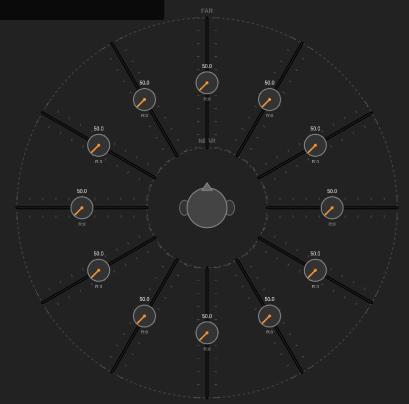
MDP – Multi Dimensional Panner
Demo: https://like.audio/MDP/
## Overview
The **Multi-Dimensional Panner (MDP)** is an advanced user interface concept designed for spatial audio mixing, object-based panning (e.g., Dolby Atmos), and complex parameter control. It extends the traditional “Linear Travelling Potentiometer” (LTP) by placing it within a free-floating, rotatable widget on a 2D plane.
CMDP: Circular Motion Displacement Potentiometer
DEMO: http://like.audio/CMDP
# CMDP: Circular Motion Displacement Potentiometer
For decades, the broadcast world was defined by physics. We built facilities based on the “Box Theory”: distinct, dedicated hardware units connected by copper. The workflow was linear and tangible. If you wanted to process a signal, you pushed it out of one box, down a wire, and into another. The cable was the truth; if the patch was made, the audio flowed.
Today, we are witnessing the dissolution of the box.
The industry is currently navigating a violent shift from Signal Flow to Data Orchestration. In this new paradigm, the “box” is often a skeuomorphic illusion—a user interface designed to comfort us while the real work happens in the abstract.
The fundamental difference lies in how information moves. In the hardware world, we “pushed” signals. Source A drove a current to Destination B. It was active and directional.
In the software world of IP and virtualization, we do not push; we share. The modern audio engine is effectively a system of memory management. One process writes audio data to a shared block of memory (a ring buffer), and another process reads it. The “wire” has been replaced by a memory pointer. We are no longer limited by the number of physical ports on a chassis, but by the read/write speed of RAM and the efficiency of the CPU.
This transition forces us to confront the chaos of computing. Hardware audio is isochronous—it flows at a perfectly locked heartbeat (48kHz). Software and cloud infrastructure are inherently asynchronous. Packets arrive in bursts; CPUs pause to handle background tasks; networks jitter.
The modern broadcast engineer’s challenge is no longer just “routing audio.” It is artificially forcing non-deterministic systems (clouds, servers, VMs) to behave with the deterministic precision of a copper wire. We are trading voltage drops for buffer underruns.
Perhaps the most radical shift is in topology. The line from Point A (Microphone) to Point B (Speaker) is no longer straight.
We are moving toward a “Point A → Cloud → Point Z → Point B” architecture. The “interface layer” is now a complex orchestration of logic that hops between cloud providers, containers, and edge devices before ever returning to the listener’s ear. The signal might traverse three different data centers to undergo AI processing or localized insertion, creating a web of dependencies that “Box Thinking” can never fully map.
The era of the soldering iron is giving way to the era of the stack. We are no longer building chains of hardware; we are architecting systems of logic. The broadcast facility of the future isn’t a room full of racks—it is a negotiated agreement between asynchronous services, sharing memory in the dark.
Input Channel Types
Architecting a Scalable, Headless Audio Console in Rust
In the world of professional audio—spanning broadcast, cinema, and large-scale live events—the mixing console is the heart of the operation. Traditionally, these have been massive hardware monoliths. Today, however, the industry is shifting toward headless, scalable audio engines that run on standard server hardware, controlled remotely by software endpoints.
This article proposes the architecture for Titan-96k, a scalable, 32-bit floating-point audio mixing engine written in Rust. It is designed to handle everything from a simple podcast setup to complex 7.1.4 immersive audio workflows, controlled entirely via MQTT.

February is Toronto AES Audio Engineering Society Member showcase….
The **Linear Travelling Potentiometer (LTP)** is a hybrid user interface widget designed to save screen real estate while maximizing control density. It integrates a rotary knob directly onto the cap of a linear fader, allowing simultaneous control of two related parameters (e.g., Level and Pan, or Send Level and Send Pan) in a single compact footprint.
Back in 2013, I presented a concept at the AES Toronto meeting called the “Linear Traveling Potentiometer” (LTP).
demo: https://like.audio/LTP/
The idea was simple but mechanically complex: Combine a linear fader and a rotary potentiometer into a single, fluid control. Two motions, one component.
I even had a prototype in a “black bag” that I let people feel without seeing. The goal was to control intensity (volume) and position (pan) simultaneously—a single-point coordinate system for surround sound and spatial audio.
For years, this existed mostly as hardware prototypes and sketches. But the vision never went away.
Now, nearly 15 years later, I have finally recreated my vision purely in software. Click, grab it like a fader… Move up for volume and sideways to pan…
I’ve brought the “Two in One” concept to life digitally. No moving parts, just the physics of the original idea translated into code.
It’s been a long road from that first presentation to this software build. Sometimes the technology just needs to catch up to the idea.

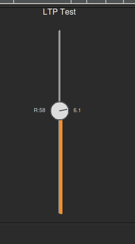

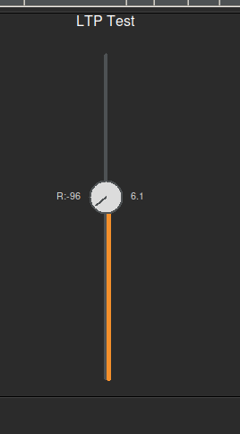
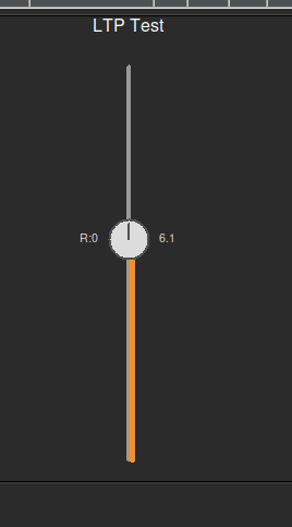
## Core Concepts
### 1. Hybrid Control
* **Linear Fader (Y-Axis):** The vertical position of the cap controls the primary value (typically Volume, Level, or Depth).
* **Rotary Knob (Rotation):** A knob embedded in the fader cap controls a secondary value (typically Pan, Param, or Intensity).
* **Unified Interaction:** Both controls are accessible from the same visual element, reducing mouse travel and UI clutter.
### 2. Interaction Modes
The LTP supports distinct interaction modes to prevent accidental changes:
* **Standard Mode:**
* **Drag Handle:** Adjusts Linear Value only.
* **Alt/Option + Drag:** Adjusts Rotary Value only (Linear position is locked).
* **Scroll:** Fine-tune Linear Value.
* **Alt/Option + Scroll:** Fine-tune Rotary Value.
* **Freestyle Mode:**
* Dragging the handle adjusts **BOTH** Linear and Rotary values simultaneously based on 2D mouse movement. This allows for gestural control (e.g., “throwing” a sound into a corner).
* **Pan Latch:**
* **Double-Click** the cap to engage “Pan Latch”.
* In this state, horizontal mouse movement adjusts the Rotary value without needing to hold a modifier key.
* Click or drag again to disengage.
### 3. Visual Feedback
* **Linear:** Position of the cap along the vertical track.
* **Rotary:** Orientation of the indicator line on the cap.
* **Active State:** The knob glows (default blue/orange) when Rotary control is active (via modifier, latch, or freestyle mode).
* **Pointer:** When adjusting rotation, the indicator line extends (10x length) to provide precise visual feedback, then retracts on release.
## Use Cases
* **Channel Strips:** Volume (Linear) + Pan (Rotary).
* **Effect Sends:** Send Level (Linear) + Pre/Post Toggle or Send Pan (Rotary).
* **Synthesizers:** Cutoff (Linear) + Resonance (Rotary).
* **Spatial Audio:** Distance (Linear) + Azimuth (Rotary – mapped to circular motion).
## Implementations
### HTML5 Demo (`index.html`)
A standalone web-based demonstration using HTML5 Canvas.
* **Features:** Multi-touch support (1 finger slide, 2 finger twist/pan), keyboard modifiers, responsive layout.
* **Theme:** Dark mode with high-contrast UI.
## The Open Concept License
This project is released under **The Open Concept License**.
* **Freedom:** You are free to use, modify, and distribute this work.
* **Attribution:** Explicit credit to **Anthony Kuzub** must be given in all derivative works.
* **Nomenclature:** Implementations must strictly use the terms **LTP (Linear Travelling Potentiometer)**, **GCA (Ganged Controlled Array)**, and **MDP (Multi-Dimensional Panner)** where applicable.
* **Warranty:** Provided “As Is” without warranty.
*(See the full license text in the application footer or source code.)*
High-Throughput Instrument Control Protocol
In the world of instrument automation (GPIB, VISA, TCP/IP), the primary bottleneck is rarely bandwidth—it is latency. Every command sent to a device initiates a handshake protocol that incurs a time penalty. When managing complex systems with hundreds of data points, these penalties accumulate, resulting in “bus chatter” that freezes the UI and blocks other processes.

The Great Decoupling is Here.
Splinkler is a specialized control connection manager designed specifically for decoupled architectures.
Splinker:
1. Splicing Control: The Need for Speed
2. Linking Feedback: The Need for Awareness

💡 The Mixer, My Grandfather, and the Looming Crisis of Unfixable Electronics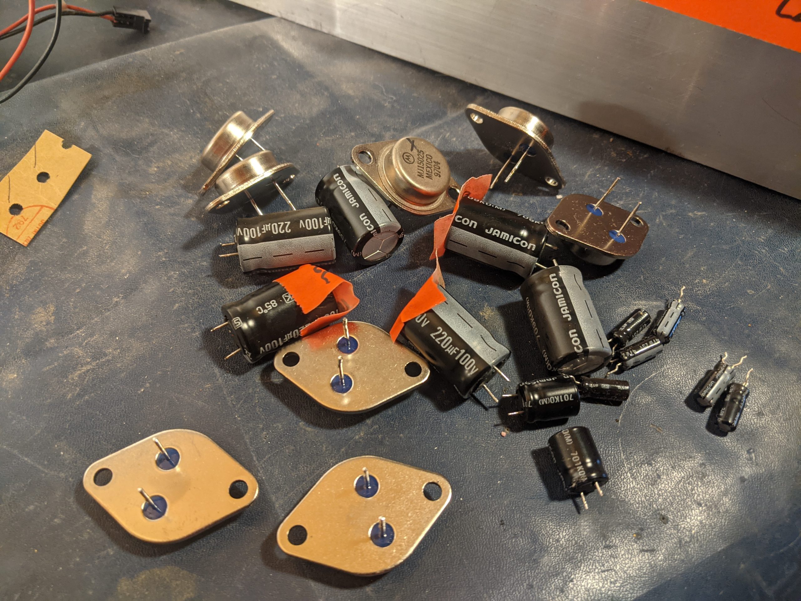

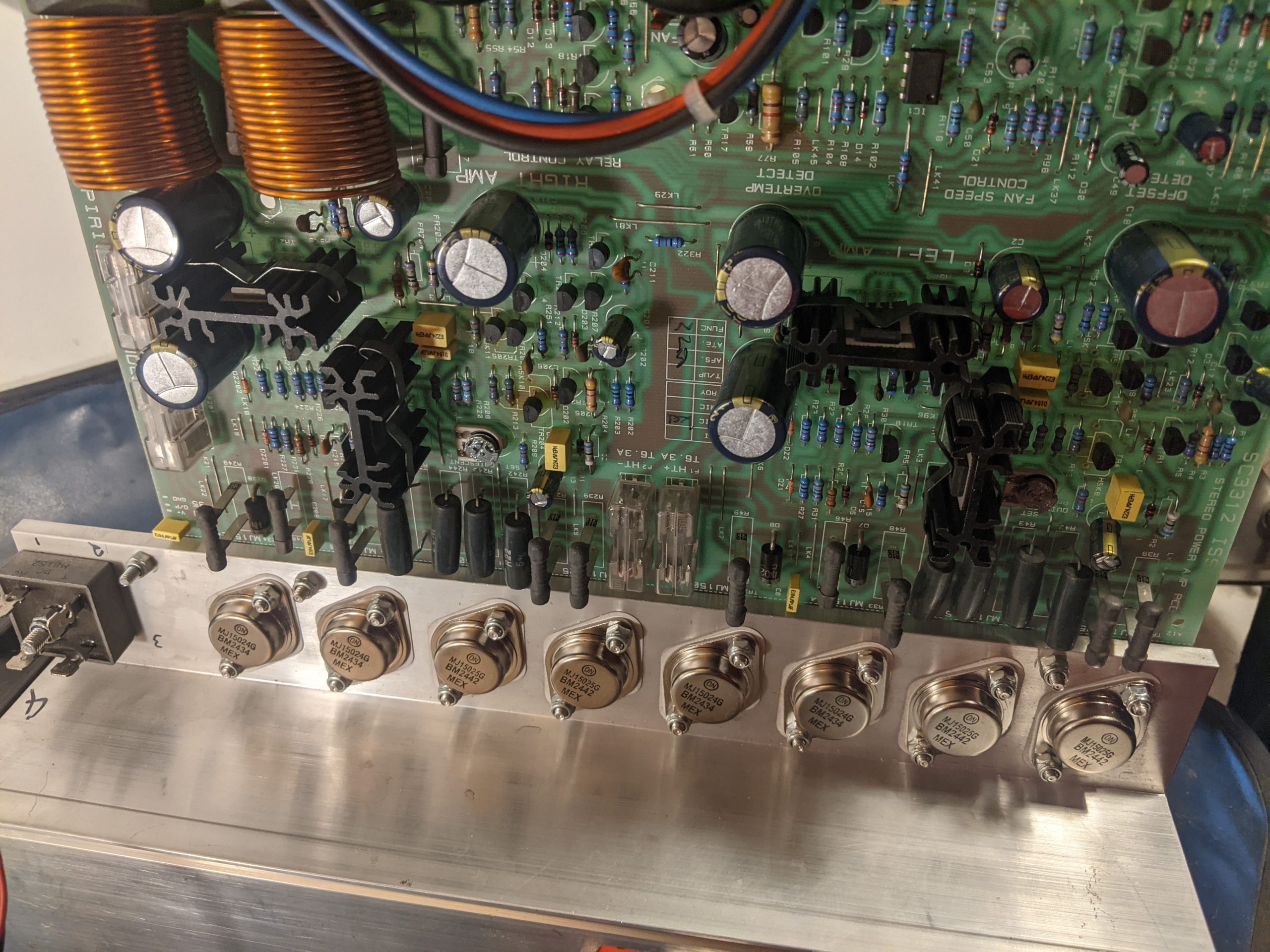
My weekend project—a powered mixer for a friend—was a powerful, hands-on lesson in the changing nature of electronics and the fight for the Right to Repair.
For a friend, I made an exception to my usual “no bench work” rule. The diagnosis was classic: a blown channel, likely from speakers incorrectly wired in parallel. Instead of a minimal patch job, I opted for a full refurbishment, the way I was taught: new, high-quality Panasonic FC caps and fresh, matched transistors. A labour of love, not profit. Continue reading


